
Creating a Machine Learning Deep CNN Image Classifier for Ants
or how to take a 3 hour task and turn it into a 50 hour task

Check out my GitHub repository to see my model.
Introduction
If you have ever used the mobile application Seek, you have probably used the functionality it provides that can help you identify plants and animals found in the world around us. It does a pretty good job, and it can help you identify a whole host of different types of plants and animals. One area where it struggles however, is in identifying ant species. With an estimated 22,000 species, ants are mind-bogglingly speciose and there just isn’t much data that has been fed into these models that allows for easy identification.
While working as a myrmecologist, I have firsthand experience with the struggles of identifying ants in the field without any tools such as a pinning board or microscope. While this (skill) issue became less prevalent as I got better at identifying ants, it always stuck in my mind, wouldn’t life be so much easier if I could just feed some images into a model that could accurately predict what ants they were. And so I embarked on the task of creating such a model- or at least creating one to the best of my abilities. The key problem for my purposes was to identify the ant Pheidole pilifera from other Lasius sp. found in the same habitat. One thing I had going for me was that Pheidole pilifera are the ONLY Pheidole found in the entire field site! So if I could get a model to identify Pheidole from Lasius, I would by design find the species of Pheidole I was looking for.
Sourcing my data
The largest challenge when creating a machine learning model is typically sourcing the data. Originally, I thought of using a bot that would scrape Google Images, but that idea soon died once I realized how messy the results from a Google search of “Myrmica rubra worker” were. There were images of other species, images with huge watermarks, and cartoon representations to name a few issues. While browsing AntWiki I realized I could get a bot to scrape their website for specimen images instead. While there weren’t a ton of images, it was a start. I then quickly realized these images all were sourced from a site called AntWeb, run by the California Academy of Sciences. This website was the jackpot - there were thousands of specimen images, mounted and photographed to taxonomic perfection. I quickly created a bot to scrape lower resolution images into my drive and I was off!
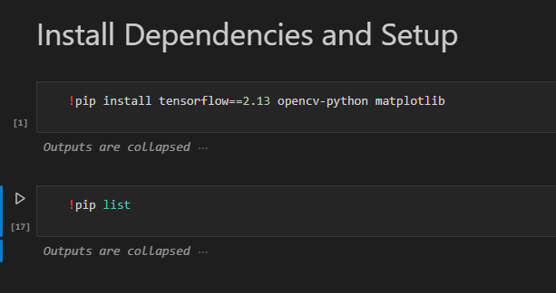
Installing dependencies
The first hurdle of building the model came when I realized TensorFlow, the library I would use to build the model was no longer supported on native Windows devices. In theory it could work on an older version of Tensorflow, but I deemed it would be not worth my time, especially since it would not make use of my GPU when generating the model. This issue was (painstakingly over ~16 hours due to some other issues that came with setting up the required environments) circumvented through the use of WSL2.
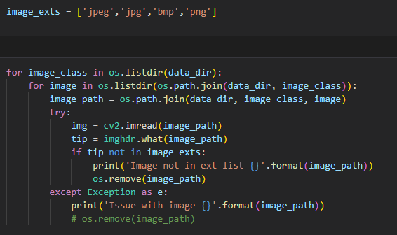
Pruning images
Once I had my dependencies and my data, the next thing I had to do was prune my data to remove any anomalies. I automated this using cv2 and imghdr after which I gave my data a cursory glance over once.
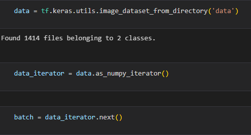
Load/Preprocess Data
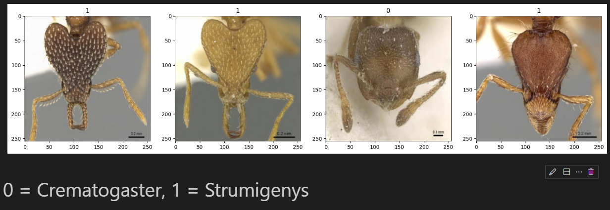
I used Keras (Python interface for artificial neural networks) to organize my data. Keras is a really powerful tool that allowed me to shuffle my data, create my batches, and resize my images for the model (256, 256). Each point of data (photo) is then stored as an array of two values. Array[0] represents the image data and Array[1] represents the data category.
When you load in a image representation in RGB channels for TensorFlow, the values are going to range from 0 to 255. When building deep learning models, you want to optimize these values into a range of 0 to 1. This enables you to train these models much faster. This scaling can be done simply by just dividing the data values by 255.
data = data.map(lambda x,y: (x/255, y))
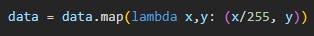
This is done as shown above. In this case x is the image data and y is the target label or the data category.
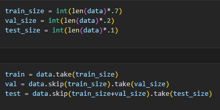
Next we split the dataset into training, validation, and testing sets. The partitioning of the dataset can be fine tuned, but for my purposes I went with 70% for testing, 20% for validation, and 10% for testing. This was done by taking the length of my dataset and multiplying it by my chosen decimal value.
Building the model
Finally! Onto the good bit. The data is processed and we are ready for liftoff. But again, first we must do some prep in the form of importing dependencies.
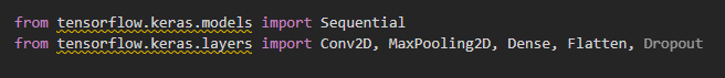
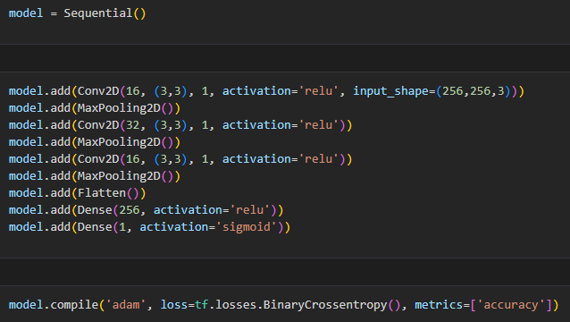
Lets go over our architectural decisions. First we call an instance of Sequential into a variable model. Then we add in our layers, which is where the magic happens. We have three sets of convolution and max pooling layers. Looking at our first set as an example:
model.add(Conv2D(16, (3,3), 1, activation='relu', input_shape=(256,256,3)))
The convolution has 16 filters that are 3 pixels by 3 pixels in size. The 1 refers to the stride, which is the amount the filter moves each time. The activation in this case is using a Rectified Linear Unit (ReLU). This basically converts all values below 0 into 0 while preserving all positive values. MaxPooling2D then condenses the data down by half for the next layer.
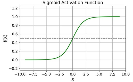
After two more sets of these layers, we flatten the data using Flatten( ). This data is then condensed further using Dense( ). These last two layers are fully-connected layers. The first one has 256 neurons with a ReLU activation and the last layer has a sigmoid activation. This final sigmoid layer converts the output of the model into a single layer that represents either 0 or 1. The values 0 and 1 map to our two image classes!
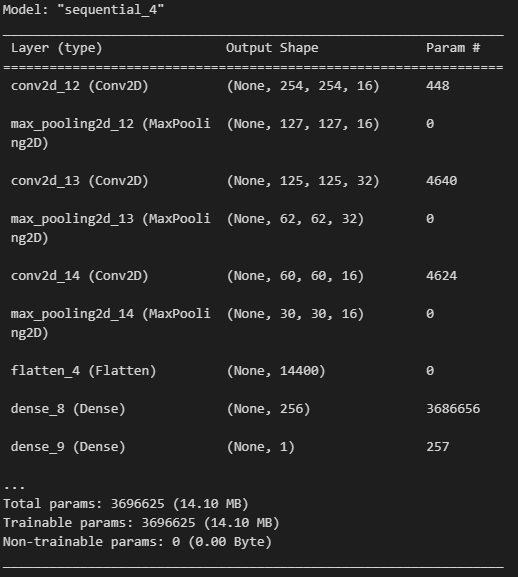
And that should be it for building the model! by using
model.summary()
we can get a quick overview of what the model we built looks like:
Training the model
Finally we can fit the model:
hist = model.fit(train, epochs=15, validation_data=val, callbacks=[tensorboard_callback])
fit() is the training component while predict() is the predictive component we will use later.
Our epochs represents how long we will train for. One epoch is equivalent to running through our data once.
validation_data is the data set we use to evaluate our model
The tensorboard_callback is responsible for creating logs for the training process (more info in the GitHub repo).
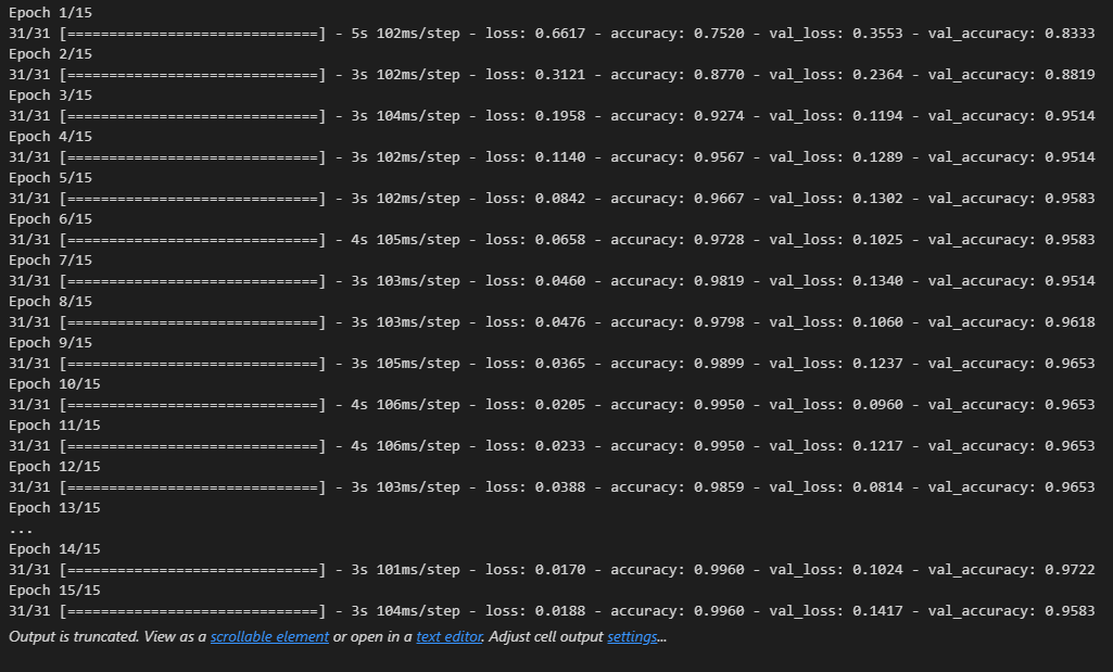
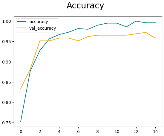
Once we train the model, we can visualize its performance with respect to each epoch.
And that should be it for making the model!
Finishing touches
You can evaluate the model using the Precision, Recall, and BinaryAccuracy packages from tensorflow.keras.metrics. More details can be found in the Jupyter Notebook in the Github repo.
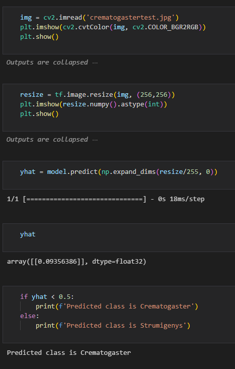
Additionally you can test (or use!) the model by using model.predict() (or in our case hist.predict() ). The value you get from the output will be between 0 and 1 as per our sigmoid function. This value will predict the class of your image!
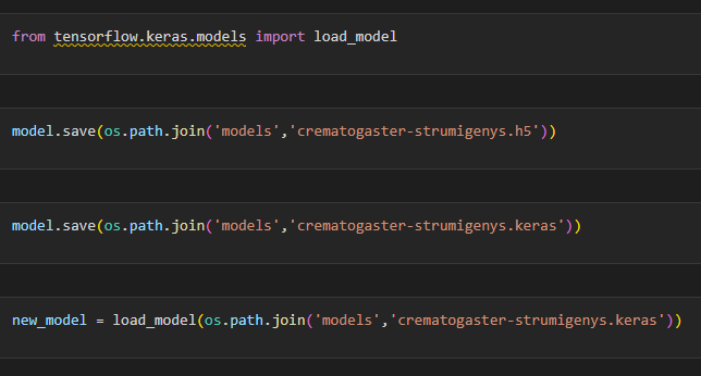
From here you can save the model using save() as either a h5 file or a keras file. I believe h5 will be deprecated soon so keras is probably your best bet. You can load saved models using from load_model() from tensorflow.keras.models
Thank you for reading! I hope this post helped you with your own model!